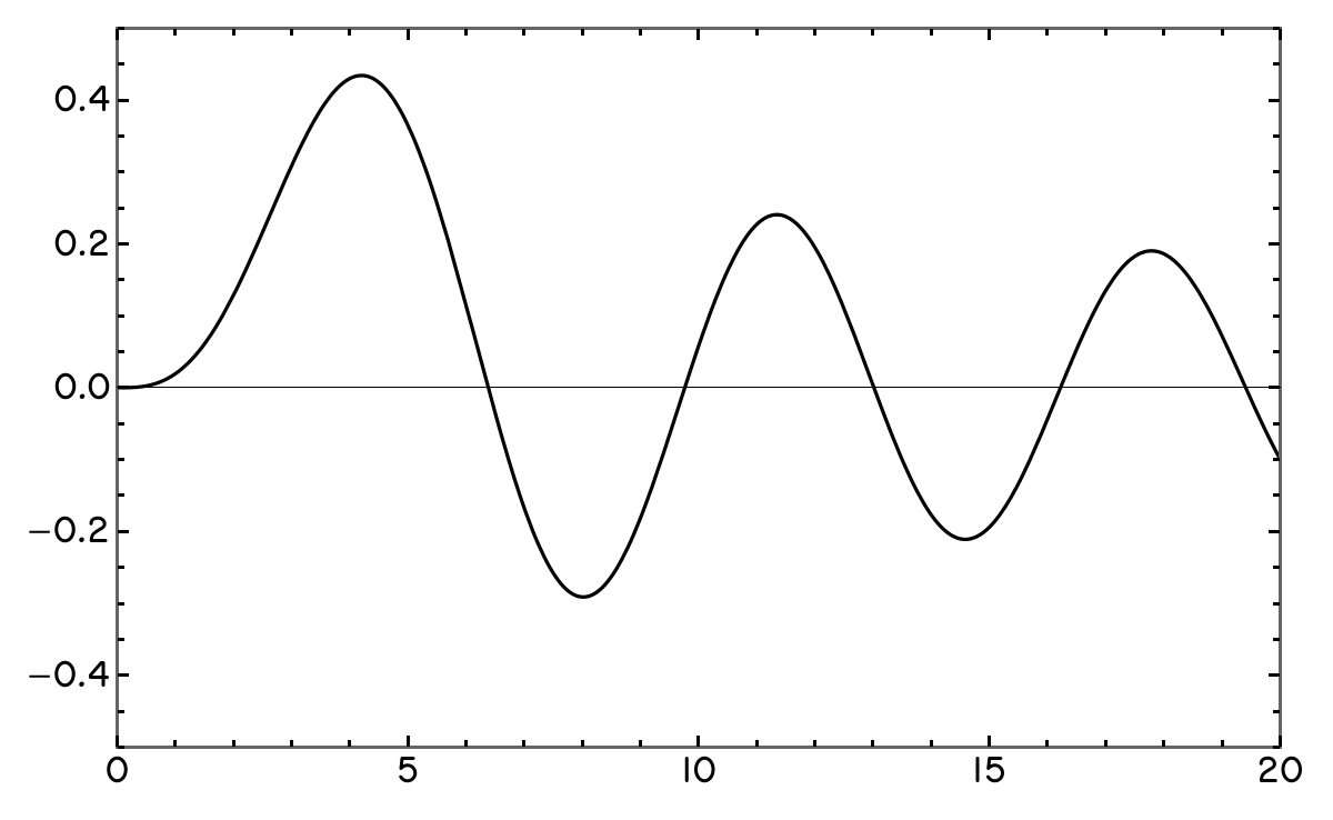
I’ve always had a soft spot for the graphs and diagrams found in Cold-War-era technical literature: chunky tick marks, thick black lines drawn with French curves, stencil letters with their telltale rounded tips and constant stroke weight. A few months ago, I set out to recreate this style in Mathematica, and I’ve been quite pleased with the result.
The code below creates a new theme called “1974”, based on Mathematica’s built-in “Monochrome” theme, which you can then pass to plotting functions via the PlotTheme option. This theme requires installing the Routed Gothic typeface.
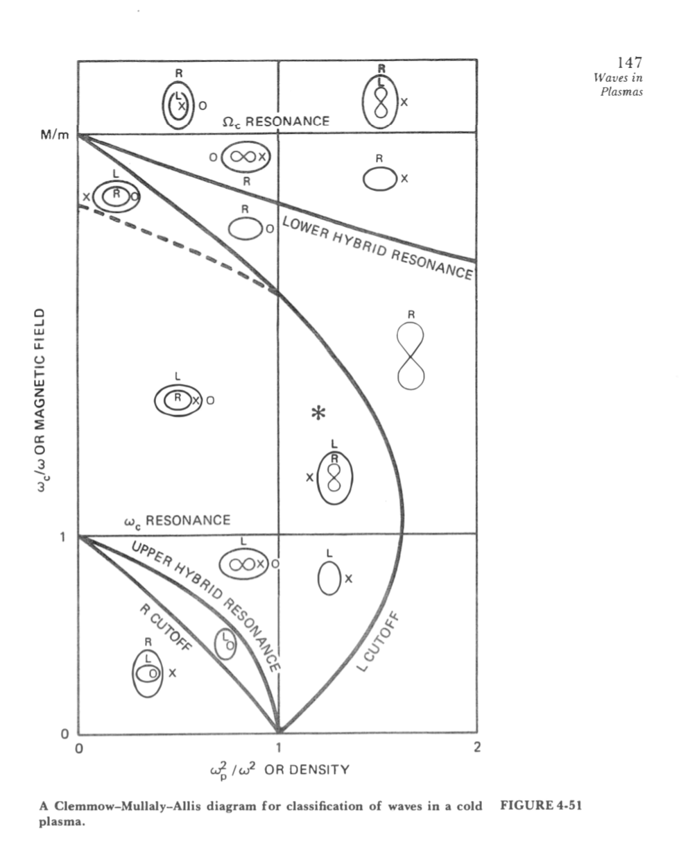
It’s named for the publication year of Francis F. Chen’s Introduction to Plasma Physics, a book with many wonderful examples of these graphics:
Code:
Link to the full example notebook.
Mathematica’s internal plotting functions aren’t publicly documented, but thanks to the work of StackExchange sleuths, some Claude prompting, and careful chaining of ClearAttribute and Definition, I’ve figured out a reasonably robust method to define my own themes:
ClearAll[AddDerivedTheme];
(* Creates a new PlotTheme based on an existing one *)
(* getCustomOpts should take in a string (the name of a plotting function) and return a list of rules *)
AddDerivedTheme[newTheme_String, baseTheme_String, getCustomOpts_] :=
    Module[{att},
        att = Attributes[Charting`ResolvePlotTheme];
        ClearAttributes[Charting`ResolvePlotTheme, att];
        Charting`ResolvePlotTheme[newTheme, f_] :=
            Module[{baseRules, overrides},
                overrides = Flatten[getCustomOpts[f]];
                baseRules = Charting`ResolvePlotTheme[baseTheme, f];
                Join[overrides, DeleteCases[baseRules, Rule[Alternatives @@ Keys[overrides], _]]]
            ];
        SetAttributes[Charting`ResolvePlotTheme, att];
    ];
(This has been tested in Mathematica 15.0.11 and will probably work in v14 as well. Some older Mathematica versions might require you to replace Charting`ResolvePlotTheme with the lower-level function System`PlotThemeDump`resolvePlotTheme—note that the lowercase r is not a typo).
Defining theme rules for “1974”:
AddDerivedTheme[
    "1974",
    "Monochrome",
    p |-> {
        (* same options for all plots, but you can break this up if you want
           different opts for different top-level plotting functions. *)
        BaseStyle  -> Directive[FontFamily -> "Routed Gothic", Black, FontSize -> 14],
        LabelStyle -> Directive[FontFamily -> "Routed Gothic", Black],
        TicksStyle -> Directive[FontSize -> 16],
        FrameStyle -> Directive[FontSize -> 16, AbsoluteThickness[1.5]],
        Frame -> True,
        PlotRangePadding -> None
    }
];

(* Mathematica's plotting infrastructure makes it hard to style legends in theme
   definitions. I got around this by defining a helper function that I can pass
   to LineLegend via the LegendFunction option. *)
LegendPostscript["1974"] := Framed[#,
    RoundingRadius -> 0,
    FrameMargins -> 0,
    BaseStyle -> Directive[FontSize -> 14, FontFamily -> "Routed Gothic"]
]&;
The new theme in action:2
(* Graph at the top of this page: *)
Plot[BesselJ[3, x], {x, 0, 20}, PlotTheme -> "1974", PlotRange -> {-1/2, 1/2}, ImageSize -> Large]

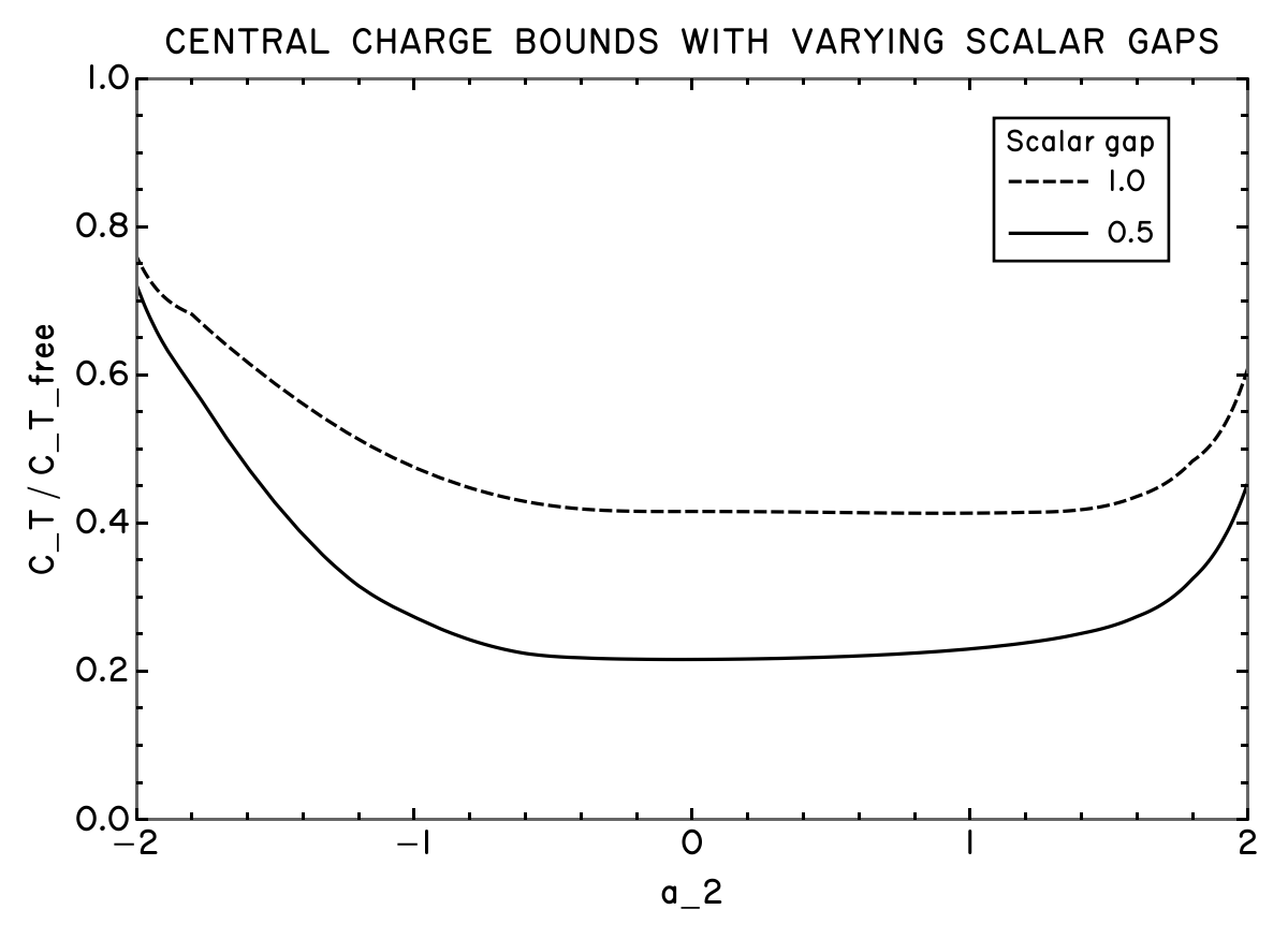
(* A more detailed example: *)
Plot[
    {Interpolation[testData1][x], Interpolation[testData2][x]},
    {x, -2.1, 2.1},
    PlotRange -> {{-2, 2}, {0, 1}},
    AspectRatio -> 2/3,
    PlotLabel -> "CENTRAL  CHARGE  BOUNDS  WITH  VARYING  SCALAR  GAPS",
    FrameLabel -> {"a_2", "C_T / C_T_free"},
    PlotTheme -> "1974",
    Axes -> None,
    PlotLegends -> Placed[
        LineLegend[
            {"0.5", "1.0"},
            LegendLabel -> "Scalar gap",
            LegendLayout -> "ReversedColumn",
            LegendFunction -> LegendPostscript["1974"]
        ],
        {{0.85, 0.85}, {0.5, 0.5}}
    ],
    ImageSize -> Large
]
-
Technically “Wolfram Notebook 15.0.1,” or whatever it’s called now. ↩︎
-
The data for the last plot comes from an attempt to reproduce some of the bounds in https://arxiv.org/abs/1705.04278. It’s from an old and buggy version of my code, so please avoid inferring anything from it. ↩︎
Comments
Comments are hosted on Bluesky. Reply to this post's Bluesky thread to join the discussion.